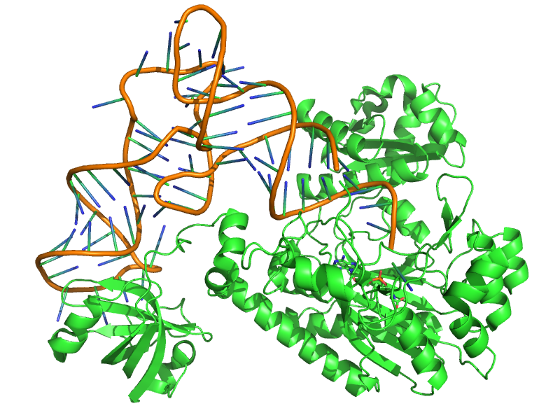
The objective of the TP is to study by molecular modeling the specific recognition between the aspartyl-tRNA synthetase and its substrate Asp. We will try to evaluate the specificity by comparing the binding of the ligands Asp and Asn. We will then seek to identify and model mutations in the active site that could favor the binding of Asn instead of Asp. This is a first step towards an engineering of the genetic code.

Aminoacyl-tRNA synthetases (aaRS) are an enzyme family implicated in protein synthesis. They are involved in translation by allowing the binding of an amino acid to its transfer RNA. They are very specific of the amino acid concerned and corresponding transfer RNA. Thus there exists one for each amino acid.
We will be interested particularly in the aspartyl-tRNA synthetase (AspRS), the goal being to perform point mutations of this enzyme in order to reduce its affinity for its natural ligand aspartate and favor its binding to asparagine.
For that, we will consider the problem in terms of protein sequences and structures. The study includes three steps:
This analysis will lead to propose judicious mutations of the active site, allowing to modify the AspRS specificity by favoring Asn binding over Asp.
The E. coli AspRS has three domains: the tRNA anticodon binding domain, the catalytic site domain, and a third one inserted into the catalytic site domain.
Launch a BLAST search. What types of proteins are found?
Identify strongly conserved regions that can correspond to the active site. Choose some positions that seem distinctive of the AspRS and of Asp binding.
Which strategy have you employed? Which mutations do you propose to modify the AspRS affinity for aspartate and asparagine?
With the informations previously obtained, propose judicious mutations to modify the AspRS affinity for aspartate and asparagine. We will try to test several of them in the next step of modeling.
Does the active site examination lead you to modify your mutation propositions made from the sequences?
Can we use the structure to verify the sequence alignment?
This is the most ambitious and complex part of the TP. There are two steps:
We will follow this protocol with the XPLOR program:
The PDB files must comply with a particular format to be readable by XPLOR. The segment name has to be written on 4 characters in columns 73-76. We also note that the 3-letter code of histidines has been changed from HIS to HIE. There indeed exists 3 possible protonation states for histidines and it is necessary to tell XPLOR which state is chosen among HID, HIE, or HIP (see the topology file amber.rtf for the definition of these states).
Does the HIE protonation state chosen for all histidines seem reasonable to you? If in doubt, try other protonation states and evaluate the impact on the results.
xplor < build.inp > build.out
xplor < minimize.inp > minimize.out
xplor < energy.inp > energy.out
What is the affinity of the AspRS protein for the Asp ligand?
What is the affinity of the AspRS for Asn?
Experimentally, the wild-type enzyme binds Asp considerably stronger than Asn, with an association free energy difference of more than 7 kcal/mol. Do you find the same tendency?
A simple mutation (for example Asp→Asn or Gln→Glu) can be realized by editing the PDB file, as explained for the ligand.
A more complex mutation can be performed with the SCWRL program. The mutation choice (for example R10K) is done by replacing in the asprs.seq file the one-letter code of the native amino acid in lowercase by the code of the amino acid chosen for the mutation in uppercase (for example replacing the lowercase ``r'' in position 10 by an uppercase ``K'').
We then launch the SCWRL program as follows:
scwrl -s asprs.seq -i asprs.wt.pdb -o asprs.pdb > scwrl.out
Compare the mutated structure obtained asprs.pdb with the native structure asprs.wt.pdb.
It is recommended to work in a separate folder for each mutant.
In order to use the structure mutated by SCWRL with XPLOR, it must be ensured that it is correctly formatted. For that, we will use the pdb2xplor program as follows:
pdb2xplor asprs.pdb A PROT > asprs.xplor.pdb
What are the affinities for Asp and Asn obtained with the mutated protein?
Have you succeeded in inverting the specificity?
Interpret structurally the effect of the mutations.
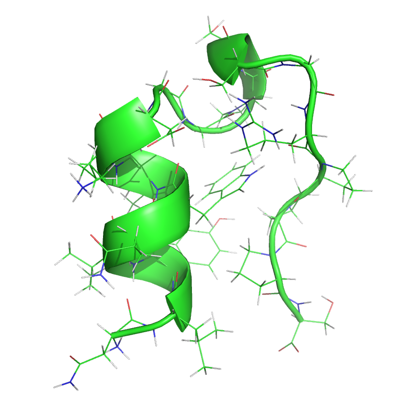
The objective of the TP is to study the structure and stability of a small protein, the Trp-cage.
 ↔
↔
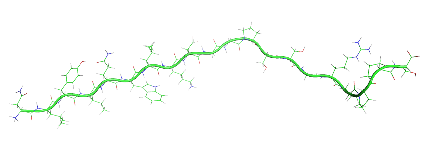
Trp-cage is a small artificial protein of 20 amino acids, which has been designed to fold easily. Its amino acid sequence is NLYIQWLKDGGPSSGRPPPS. The protein folding problem is one of the most important challenges of structural bioinformatics. It consists in predicting the three-dimensional structure of a protein from the sequence information alone.
We will employ the methods of molecular mechanics to model the Trp-cage.
xplor < build.inp > build.out
This script builds a model of the Trp-cage with XPLOR and performs an energy minimization to improve the geometry.
Inspect the output file and visualize the structures produced.
xplor < md.inp > md.out
This script performs a molecular dynamics of the Trp-cage during 20ps, assigning random initial velocities and then maintaining the temperature at 300K.
Inspect the output file and track the energy and temperature as a function of time.
xplor < traj2mpdb.inp > traj2mpdb.out
This script converts the format of the trajectory produced from DCD to multiple PDB.
We can then visualize the trajectory with PyMOL by loading it as follows:
load md.multi.pdb, multiplex=0
xplor < analyze.inp > analyze.out
This script reads the produced trajectory (md.dcd) and performs structural or energetic calculations at each step. The results are written in a text file (md.dat). Represent them graphically.
The analyses included in the script are only examples, it is your task to add more relevant ones with the help of the XPLOR documentation.
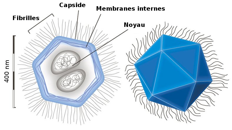
Mimivirus is a giant DNA virus. It is larger than many bacteria, and can itself be infected by other viruses. It was discovered that mimivirus possesses certain genes for proteins involved in translation, absent in other viruses that use the host cell's machinery to multiply. These discoveries have fuelled debate about the boundary between living and inert matter.
Homology modeling aims at building a model of the unknown structure of a target protein, knowing its sequence and the structure of another template protein of homologous sequence. The method can be decomposed into four steps:
The aim of this work is to propose the best possible structural model (criteria to be defined) of mimivirus tyrosyl-tRNA synthetase (its structure is assumed to be unknown) by homology modelling with the Modeller program.
Retrieve the sequence of mimivirus tyrosyl-tRNA synthetase in FASTA format in UniProt (http://www.uniprot.org) database.
Carefully select a structure to be used as a guide for homology modeling (of course, we won't use the structure of mimivirus tyrosyl-tRNA synthetase, which we assume to be unknown). Retrieve this structure in PDB format.
Convert query sequence from FASTA to PIR format (http://salilab.org/modeller/manual, File formats, Alignment file (PIR)) with which Modeller works. Example of a sequence in PIR format:
>P1;TvLDH
sequence:TvLDH::::::::
MSEAAHVLITGAAGQIGYILSHWIASGELYGDRQVYLHLLDIPPAMNRLTALTMELEDCAFPHLAGFVATTDPKA
AFKDIDCAFLVASMPLKPGQVRADLISSNSVIFKNTGEYLSKWAKPSVKVLVIGNPDNTNCEIAMLHAKNLKPEN
FSSLSMLDQNRAYYEVASKLGVDVKDVHDIIVWGNHGESMVADLTQATFTKEGKTQKVVDVLDHDYVFDTFFKKI
GHRAWDILEHRGFTSAASPTKAAIQHMKAWLFGTAPGEVLSMGIPVPEGNPYGIKPGVVFSFPCNVDKEGKIHVV
EGFKVNDWLREKLDFTEKDLFHEKEIALNHLAQGG*
The Modeller program is launched as follows:
modeller file.py
Align the query sequence with the sequence of the selected guide structure by adapting the align2d.py script.
modeller align2d.py
The alignment produced is written in PIR, PAP, and FASTA formats. Examine these files.
Model by homology the target structure by adapting the model-single.py script.
modeller model-single.py
A summary including the PDB file names of the models produced as well as the value of the Modeller energy function and the DOPE score for each model can be found at the end of the output file (model-single.log). Examine the models produced with PyMOL.
Evaluate the models generated in the previous step by adapting the evaluate_model.py script.
modeller evaluate_model.py
This script allows a more detailed evaluation of the models produced by calculating the DOPE score for each position of the alignment. Plot the DOPE score as a function of position (columns 1 and 42) for the different models.
For further information:
Modeller tutorial: http://salilab.org/modeller/tutorial/basic.html
Modeller manual: http://salilab.org/modeller/manual
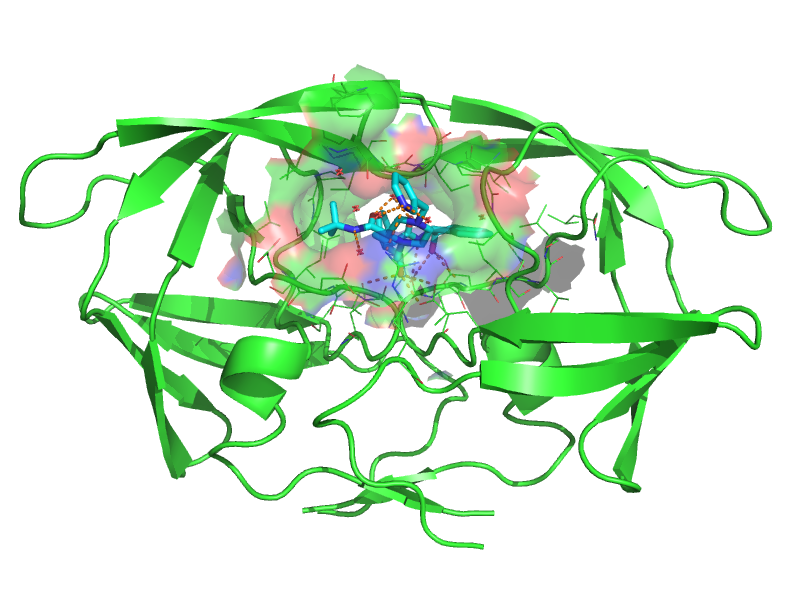
AutoDock is a suite of tools for molecular docking. Docking involves predicting how ligands, such as substrates or potential drugs, bind to a receptor with a known three-dimensional structure.
The AutoDock docking procedure comprises two main steps:
We will also be using a graphical interface called AutoDockTools (ADT) to facilitate docking preparation and visualize the results.
The method will be illustrated with the docking of Indinavir, an HIV-1 protease inhibitor, used as an antiretroviral in the treatment of AIDS.
AutoDock needs to know the charge and type of each atom, as well as a list of the freely rotating bonds present in the ligand.
adt
→ → → → "ind.pdb"
AutoDockTools reads the ligand and performs the following steps: calculation of Gasteiger-type atomic charges, fusion of non-polar hydrogens, assigning atomic types, detecting the number of torsional degrees of freedom.
Atomic types and charges are used in the molecular mechanics terms of AutoDock scoring function. The number of torsional degrees of freedom of the ligand determines its flexibility and is also used in the calculation of the entropy penalty of association.
→ →
The smallest rigid group in the molecule includes this atom and all the atoms connected to it by bonds without free rotation.
→ →
Bonds without free rotation are shown in red, those that could undergo a rotation but marked as inactive appear in purple, while those marked as active appear in green. Leave the default definition, which corresponds to 14 degrees of freedom.
→ →
Reduce the number of degrees of freedom to 6 ("fewest atoms") to speed up the calculation.
→ → → "ind.pdbqt"
→ → → → "hsg1.pdb"
AutoDockTools reads the receptor and, as with the ligand, performs the steps of calculating Gasteiger-type atomic charges, merging non-polar hydrogens and assigning atomic types.
Save the receptor as "hsg1.pdbqt".
It is necessary to generate an interaction map for each atomic type of ligand, plus one for electrostatics and one for desolvation.
→ → → "ind" →
→
Choose 60, 60 and 66 for the number of grid points in x, y and z directions; and 2.5, 6.5 and -7.5 for the x, y and z coordinates of the grid center position.
→
→ → → "hsg1.gpf"
The .gpf file contains the parameters for the AutoGrid program.
→ →
The AutoGrid program is executed with the previously generated parameter
file (the corresponding command line is autogrid4 -p hsg1.gpf -l hsg1.glg).
The maps produced are written to the current directory and have the .map extension.
→ → → "hsg1.pdbqt"
→ → → "ind" → →
→ →
Reduce the number of evaluations of the genetic algorithm to 250000 ("short") then click on .
→ → → "ind.dpf"
The .dpf file contains the parameters for the AutoDock program. We have chosen the Lamarckian genetic algorithm as conformational sampling method.
→ →
The AutoDock program is executed with the previously generated parameter
file (the corresponding command line is autodock4 -p ind.dpf -l ind.dlg).
→ →
→ → → "ind.dlg"
→ →
→ →
A control bar appears, allowing you to browse the conformations found by docking. Conformation 0 is the starting one.
Change options by clicking on the "&" button on the bar.
Select "Show Info" and examine the energy terms displayed.
Browse through the conformations.
Change ligand and receptor representation and coloring modes. For example, you could display the molecular surface of the receptor to visualize shape complementarity with the ligand.
Use the control bar to position yourself on the best conformation.
A new object "ind_conf_1" is created.
Select this object.
Save the structure in a PDB file
→ → → "ind_conf_1.pdb" →
The experimental structure of the complex has the PDB code 1HSG.
Documentation en ligne de XPLOR 3.1
Linux installation in a virtual machine
Linux Command Line Cheat Sheet